In Agile vs. Waterfall Programming and the Value of Having a Theoretical Framework, I explained that back in the 1950s and 1960s IT professionals used an Agile methodology to develop software because programs had to be very small to fit into the puny amount of memory that mainframe computers had at the time. Recall that the original UNIVAC I came out in 1951 with only 12 KB of memory. By 1970, mainframe computers typically only had about 1 MB of memory that was divided up into a number of fixed regions by the IBM 360-MFT operating system. Typically, the largest memory region was only 256 KB. Now you really cannot do a lot of logic in 256 KB of memory so applications in the 1960s consisted of lots of very small programs in a JCL job stream that used many tapes for input and output. Each step in the job stream had a very small program that would read the tapes from the previous job step, do some processing on the data, and then write out the processed data to tapes for the next step in the JCL job stream. The output tapes were then used as input for the next step in the JCL job stream. For more on tape processing see: An IT Perspective on the Origin of Chromatin, Chromosomes and Cancer.
So this kind of tape batch processing easily lent itself to the prototyping of the little programs in each job step. Developers would simply "breadboard" each little step by trial and error like they used to do on the Unit Record Processing machines of the 1950s that were programmed by physically rewiring the plugboards of each Unit Record Processing machine in a job stream. The Unit Record Processing machines would then process hundreds of punch cards per minute by routing the punch cards from machine to machine in processing streams.

Figure 1 – In the 1950s, Unit Record Processing machines like this card sorter were programmed by physically rewiring a plugboard.

Figure 2 – The plugboard for a Unit Record Processing machine. Programming a plugboard was a trial and error process that had to be done in an Agile manner. This Agile programming technique carried over to the programming of the small batch programs in a tape batch processing stream.
To get a better appreciation for how these small programs in a long tape batch processing stream worked, and how they were developed in a piecemeal prototyping manner, let's further explore tape batch processing.
Batch Tape Processing and Sequential Access Methods
One of the simplest and oldest sequential access methods is called QSAM - Queued Sequential Access Method:
Queued Sequential Access Method
http://en.wikipedia.org/wiki/Queued_Sequential_Access_Method
I did a lot of magnetic tape processing in the 1970s and early 1980s using QSAM. At the time we used 9 track tapes that were 1/2 inch wide and 2400 feet long on a reel with a 10.5 inch diameter. The tape had 8 data tracks and one parity track across the 1/2 inch tape width. That way we could store one byte across the 8 1-bit data tracks in a frame, and we used the parity track to check for errors. We used odd parity, if the 8 bits on the 8 data tracks in a frame added up to an even number of 1s, we put a 1 in the parity track to make the total number of 1s an odd number. If the 8 bits added up to an odd number of 1s, we put a 0 in the parity track to keep the total number of 1s an odd number. Originally, 9 track tapes had a density of 1600 bytes/inch of tape, with a data transfer rate of 15,000 bytes/second. Remember, a byte is 8 bits and can store one character, like the letter “A” which we encode in the ASCII code set as A = “01000001”.

Figure 3 – A 1/2 inch wide 9 track magnetic tape on a 2400-foot reel with a diameter of 10.5 inches

Figure 4 – 9 track magnetic tape had 8 data tracks and one parity track using odd parity which allowed for the detection of bad bytes with parity errors on the tape.
Later, 6250 bytes/inch tape drives became available, and I will use that density for the calculations that follow. Now suppose you had 10 million customers and the current account balance for each customer was stored on an 80-byte customer record. A record was like a row in a spreadsheet. The first field of the record was usually a CustomerID field that contained a unique customer ID like a social security number and was essentially the equivalent of a promoter region on the front end of a gene in DNA. The remainder of the 80-byte customer record contained fields for the customer’s name and billing address, along with the customer’s current account information. Between each block of data on the tape, there was a 0.5 inch gap of “junk” tape. This “junk” tape allowed for the acceleration and deceleration of the tape reel as it spun past the read/write head of a tape drive and perhaps occasionally reversed direction. Since an 80-byte record only came to 80/6250 = 0.0128 inches of tape, which is quite short compared to the overhead of the 0.5 inch gap of “junk” tape between records, it made sense to block many records together into a single block of data that could be read by the tape drive in a single I/O operation. For example, blocking 100 80-byte records increased the block size to 8000/6250 = 1.28 inches and between each 1.28 inch block of data on the tape, there was the 0.5 inch gap of “junk” tape. This greatly reduced the amount of wasted “junk” tape on a 2400-foot reel of tape. So each 100 record block of data took up a total of 1.78 inches of tape and we could get 16,180 blocks on a 2400-foot tape or the data for 1,618,000 customers per tape. So in order to store the account information for 10 million customers, you needed about 6 2400-foot reels of tape. That means each step in the batch processing stream would use 6 input tapes and 6 output tapes. The advantage of QSAM, over an earlier sequential access method known as BSAM, was that you could read and write an entire block of records at a time via an I/O buffer. In our example, a program could read one record at a time from an I/O buffer which contained the 100 records from a single block of data on the tape. When the I/O buffer was depleted of records, the next 100 records were read in from the next block of records on the tape. Similarly, programs could write one record at a time to the I/O buffer, and when the I/O buffer was filled with 100 records, the entire I/O buffer with 100 records in it was written as the next block of data on an output tape.

Figure 5 – Between each record, or block of records, on a magnetic tape, there was a 0.5 inch gap of “junk” tape. The “junk” tape allowed for the acceleration and deceleration of the tape reel as it spun past the read/write head on a tape drive. Since an 80-byte record only came to 80/6250 = 0.0128 inches, it made sense to block many records together into a single block that could be read by the tape drive in a single I/O operation. For example, blocking 100 80-byte records increased the block size to 8000/6250 = 1.28 inches, and between each 1.28 inch block of data on the tape, there was a 0.5 inch gap of “junk” tape for a total of 1.78 inches per block.

Figure 6 – Blocking records on tape allowed data to be stored more efficiently.
So it took 6 tapes to just store the rudimentary account data for 10 million customers. The problem was that each tape could only store 123 MB of data. Not too good, considering that today you can buy a 1 TB PC disk drive that can hold 8525 times as much data for about $100! Today, you could also store about 67 times as much data on a $7.00 8 GB thumb drive. So how could you find the data for a particular customer on 24,000 feet (2.72 miles) of tape? Well, you really could not do that reading one block of data at a time with the read/write head of a tape drive, so we processed data with batch jobs using lots of input and output tapes. Generally, we had a Master Customer File on 6 tapes and a large number of Transaction tapes with insert, update and delete records for customers. All the tapes were sorted by the CustomerID field, and our programs would read a Master tape and a Transaction tape at the same time and apply the inserts, updates and deletes on the Transaction tape to a new Master tape. So your batch job would read a Master and Transaction input tape at the same time and would then write to a single new Master output tape. These batch jobs would run for many hours, with lots of mounting and unmounting of dozens of tapes.

Figure 7 – The batch processing of 10 million customers took a lot of tapes and tape drives.
When developing batch job streams that used tapes, each little program in the job stream was prototyped first using a small amount of data on just one input and one output tape in a stepwise manner.
The Arrival of the Waterfall Methodology
This all changed in the late 1970s when interactive computing began to become a significant factor in the commercial software that corporate IT departments were generating. By then mainframe computers had much more memory than they had back in the 1960s, so interactive programs could be much larger than the small programs found within the individual job steps of a batch job stream. Since the interactive software had to be loaded into a computer all in one shot, and required some kind of a user interface that did things like checking the input data from an end-user, and also had to interact with the end-user in a dynamic manner, interactive programs were necessarily much larger than the small programs that were found in the individual job steps of a batch job stream. These factors caused corporate IT departments to move from the Agile prototyping methodologies of the 1960s and early 1970s to the Waterfall methodology of the 1980s, and so by the early 1980s prototyping software on the fly was considered to be an immature approach. Instead, corporate IT departments decided that a formal development process was needed, and they chose the Waterfall approach used by the construction and manufacturing industries to combat the high costs of making changes late in the development process. This was because in the early 1980s CPU costs were still exceedingly quite high so it made sense to create lots of upfront design documents before coding actually began to minimize the CPU costs involved with creating software. For example, in the early 1980s, if I had a $100,000 project, it was usually broken down as $25,000 for programming manpower costs, $25,000 for charges from IT Management and other departments in IT, and $50,000 for program compiles and test runs to develop the software. Because just running compiles and test runs of the software under development consumed about 50% of the costs of a development project, it made sense to adopt the Waterfall development model to minimize those costs.
Along Comes NASA
Now all during this time, NASA was trying to put people on the Moon and explore the Solar System. At first, NASA also adopted a more Agile approach to project management using a trial and error approach to solve the fundamental problems of rocketry. If you YouTube some of the early NASA launches from the late 1950s and early 1960s, you will see many rocket failures blowing up in a large fireball:
Early U.S. rocket and space launch failures and explosions
https://www.youtube.com/watch?v=13qeX98tAS8
This all changed when NASA started putting people on top of their rockets. Because the NASA rockets were getting much larger, more complicated and were now carrying live passengers, NASA switched from an Agile project management approach to a Waterfall project management approach run by the top-down command-and-control management style of corporate America in the 1960s:
NASA's Marshall Space Flight Center 1960s Orientation Film
https://www.youtube.com/watch?v=qPmJR3XSLjY
All during the 1960s and 1970s NASA then went on to perform numerous technological miracles using the Waterfall project management approach and the top-down command-and-control management style of corporate America in the 1960s.
SpaceX Responds with an Agile Approach to Exploring the Solar System
Despite the tremendous accomplishments of NASA over many decades, speed to market was never one of NASA's strong suits. Contrast that with the astounding progress that SpaceX has made, especially in the past year. Elon Musk started out in software, and with SpaceX, Elon Musk has taken the Agile techniques of software development and applied them to the development of space travel. The ultimate goal of SpaceX is to put colonies on the Moon and Mars using a SpaceX Starship.

Figure 8 – The SpaceX Starship SN8 is currently sitting on a pad at the SpaceX Boca Chica launch facility in South Texas awaiting a test flight.
SpaceX is doing this in an Agile stepping stone manner. SpaceX is funding this venture by launching satellites for other organizations using their reusable Falcon 9 rockets. SpaceX is also launching thousands of SpaceX Starlink satellites with Falcon 9 rockets. Each Falcon 9 rocket can deliver about 60 Starlink satellites into low-Earth orbit to eventually provide broadband Internet connectivity to the entire world. It is expected that the revenue from Starlink will far exceed the revenue obtained from launching satellites for other organizations.

Figure 9 – SpaceX is currently making money by launching satellites for other organixations using reusable Falcon 9 rockets.
Unlike NASA in the 1960s and 1970s, SpaceX uses Agile techniques to design, test and improve individual rocket components rather than NASA's Waterfall approach to build an entire rocket in one shot.

Figure 10 – Above is a test flight of the SpaceX Starhopper lower stage of the SpaceX Starship that was designed and built in an Agile manner
Below is a YouTube video by Marcus House that covers many of the remarkable achievements that SpaceX has attained over the past year using Agile techniques:
This is how SpaceX is changing the space industry with Starship and Crew Dragon
https://www.youtube.com/watch?v=CmJGiJoU-Vo
Marcus House comes out with a new SpaceX YouTube video every week or two and I highly recommend following his YouTube Channel for further updates.
Marcus House SpaceX YouTube Channel
https://www.youtube.com/results?search_query=marcus+house+spacex&sp=CAI%253D
Many others have commented on the use of Agile techniques by SpaceX to make astounding progress in space technology. Below are just a few examples.
SpaceX’s Use of Agile Methods
https://medium.com/@cliffberg/spacexs-use-of-agile-methods-c63042178a33
SpaceX Lessons Which Massively Speed Improvement of Products
https://www.nextbigfuture.com/2018/12/reverse-engineering-spacex-to-learn-how-to-speed-up-technological-development.html
Pentagon advisory panel: DoD could take a page from SpaceX on software development
https://spacenews.com/pentagon-advisory-panel-dod-could-take-a-page-from-spacex-on-software-development/
If SpaceX Can Do It Than You Can Too
https://www.thepsi.com/if-spacex-can-do-it-than-you-can-too/
Agile Is Not Rocket Science
https://flyntrok.com/2020/09/01/spacex-and-an-agile-mindset/
Using Orbiter2016 to Simulate Space Flight
If you are interested in things like SpaceX, you should definitely try out some wonderful free software called Orbiter2016 at:
Orbiter Space Flight Simulator 2016 Edition
http://orbit.medphys.ucl.ac.uk/index.html
Be sure to download the Orbiter2016 core package and the high-resolution textures. Also, be sure to download Jarmonik's D3D9 graphics client and XRsound. There is also a button on the Download page for the Orbit Hangar Mods addon repository.
From the Orbit Hangar Mods addon repository, you can download additional software for Orbiter2016. Be careful! Some of these addon packages contain .dll files that overlay .dll files in the Orbiter2016 core package. And some of the .dll files in one addon package may overlay the .dll files of another addon package. All of this software can be downloaded from the Orbiter2016 Download page and it comes to about 57 GB of disk space! If you try to add additional addons, I would recommend keeping a backup copy of your latest working version of Orbiter2016. That way, if your latest attempt to add an addon crashes Orbiter2016, you will be able to recover from it. This sounds like a lot of software, but do not worry, Orbiter2016 runs very nicely on my laptop with only 4 GB of memory and a very anemic graphics card.

Figure 11 – Launching a Delta IV rocket from Cape Canaveral.

Figure 12 – As the Delta IV rocket rises, you can have the Orbiter2016 camera automatically follow it.

Figure 13 – Each vehicle in Orbiter2016 can be viewed from the outside or from an internal console.

Figure 14 – The Delta IV rocket releases its solid rocket boosters.

Figure 15 – The Delta IV rocket second stage is ignited.

Figure 16 – The Delta IV rocket faring is released so that the payload satellite can be released.
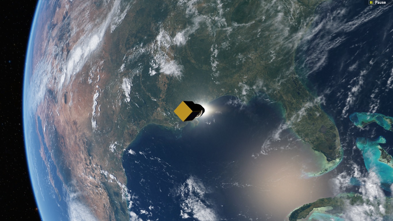
Figure 17 – The third stage is ignited.

Figure 18 – Launching the Atlantis Space Shuttle.

Figure 19 – Following the Atlantis Space Shuttle as it rises.

Figure 20 – Once the Atlantis Space Shuttle reaches orbit, you can open the bay doors and release the payload. You can also do an EVA with a steerable astronaut.

Figure 21 – Using Orbiter2016 to fly over the Moon.
Check your C:\Orbiter2016\Doc directory for manuals covering the Orbiter2016. The C:\Orbiter2016\Doc\Orbiter.pdf is a good place to start. Orbiter2016 is a very realistic simulation that can teach you a great deal about orbital mechanics. But to get the most benefit from Orbiter2016, you need an easy way to learn how to use it. Below is a really great online tutorial that does that.
Go Play In Space
https://www.orbiterwiki.org/wiki/Go_Play_In_Space
There also are many useful Orbiter2016 tutorials on YouTube that can show you how to use Orbiter2016.
Comments are welcome at scj333@sbcglobal.net
To see all posts on softwarephysics in reverse order go to:
https://softwarephysics.blogspot.com/
Regards,
Steve Johnston
No comments:
Post a Comment