In my Introduction to Softwarephysics, I explained that when I first transitioned from being an exploration geophysicist exploring for oil to become an IT professional in 1979, I decided to take all of the physics, chemistry, biology, and geology that I could muster and throw it at the problem of software in order to found a new simulated science that I called softwarephysics. The initial purpose of softwarephysics was to help me cope with the daily mayhem of life in IT that all IT professionals are quite familiar with. Then in Software as a Virtual Substance, I quickly laid out a plan for future posts on softwarephysics to cover concepts from thermodynamics, statistical mechanics, chemistry, quantum mechanics and the quantum field theories of QED and QCD that come from the Standard Model of particle physics to help explain the odd behaviors of software under load. Additionally, in Software Chaos we explored the nature of nonlinear systems and chaos theory to help explain why software is so inherently unstable. As we saw in The Fundamental Problem of Software all these factors come together to make it very difficult to write and maintain software. This is largely due to the second law of thermodynamics introducing small bugs into software whenever software is written or changed and also to the nonlinear nature of software that allows small software bugs to frequently produce catastrophic effects. In later postings on softwarephysics, I explained that the solution was to take a biological approach to software by "growing" code biologically instead of writing code. Throughout many of my posts on softwarephysics, you will also find many additional concepts from biology being put to good use to help us to better understand the apparent nature and foibles of software. But why should geology be important to softwarephysics?
Geology is important to softwarephysics because it studies the interactions between the hardware and software of carbon-based life in Deep Time on the Earth. One of the chief findings of softwarephysics is that carbon-based life and software are both forms of self-replicating information with software now rapidly becoming the dominant form of self-replicating information on the planet. For more on that see A Brief History of Self-Replicating Information. In this view, carbon-based life can be thought of as the software of the Earth's crust while the dead atoms in the rocks of the Earth's crust can be thought of as the hardware of the Earth. The rocks of the Earth's crust, and the comets and asteroids that later fell to the Earth to become part of the Earth's crust, provided the necessary hardware of dead atoms that could then be combined into the complex organic molecules necessary for carbon-based life to appear. For more on that see The Bootstrapping Algorithm of Carbon-Based Life. In a similar manner, the dead atoms within computers allowed for the rise of software. But unlike the dead atoms of hardware, both carbon-based life and computer software had agency - they both could do things. Because they both had agency, carbon-based life and computer software have both greatly affected the evolution of the hardware upon which they ran. Over the past 4.0 billion years of carbon-based evolution on the Earth, carbon-based life has always been intimately influenced by the geological evolution of the planet, and similarly, carbon-based life greatly affected the geological evolution of the Earth as well over that period of time. For example, your car was probably made from the iron atoms that were found in the redbeds of a banded iron formation. You see, before carbon-based life discovered photosynthesis, the Earth's atmosphere did not contain oxygen and seawater was able to hold huge amounts of dissolved iron. But when carbon-based life discovered photosynthesis about 2.5 billion years ago, the Earth's atmosphere slowly began to accumulate oxygen. The dissolved oxygen in seawater caused massive banded iron formations to form around the world because the oxygen caused the dissolved iron to precipitate out and drift to the bottom of the sea.

Figure 1 – Above is a close-up view of a sample taken from a banded iron formation. The dark layers in this sample are mainly composed of magnetite (Fe3O4) while the red layers are chert, a form of silica (SiO2) that is colored red by tiny iron oxide particles. The chert came from siliceous ooze that was deposited on the ocean floor as silica-based skeletons of microscopic marine organisms, such as diatoms and radiolarians, drifted down to the ocean floor. Some geologists suggest that the layers formed annually with the changing seasons. Take note of the small coin in the lower right for a sense of scale.
There are many other examples of how carbon-based life and geological processes have directly interacted and influenced each other over Deep Time as both coevolved into what we see today. Most of the Earth's crust is covered by a thin layer of sedimentary rock. These sedimentary rocks were originally laid down as oozy sediments in flat layers at the bottom of shallow seas. The mud brought down in rivers was deposited in the shallow seas to form shales and the sand that was brought down was deposited to later become sandstones. Many limestone deposits were also formed from the calcium carbonate shells of carbon-based life that slowly drifted down to the bottom of the sea or from the remainders of coral reefs. In a similar fashion, computer software and hardware have also directly interacted and influenced each other over the past 80 years or 2.5 billion seconds of Deep Time, ever since Konrad Zuse first cranked up his Z3 computer in May of 1941.

Figure 2 – Above are the famous White Cliffs of Dover. About 70 million years ago Great Britain and much of Europe were submerged under a shallow sea. The sea bottom was covered with white mud formed from the calcium carbonate skeletons of coccoliths. The coccoliths were tiny algae that floated in the surface waters and sank to the bottom during the Cretaceous period. These calcium carbonate layers were deposited very slowly. It took about 50 years to deposit an inch, but nearly 1500 feet of sediments were deposited in some areas. The weight of overlying sediments caused the deposits to become a form of limestone called chalk.
By Deep Time, I mean time spans that range from hundreds of millions to many billions of years. Geology is the only science that gives you an appreciation for Deep Time on a visceral level. Yes, astronomers and astrophysicists also deal with Deep Time but always at a great distance. It is hard for human beings to fully relate to the Deep Time experienced by stars and galaxies because they are so distant and seemingly aloof to the unaided eye. However, being able to use your rock hammer to whack some exposed rock on an outcrop that is hundreds of millions or even many billions of years old really brings Deep Time to life. Finding fossils of ancient life in those rocks that had been patiently hiding for hundreds of millions of years until you came along to free them with your rock hammer also profoundly makes Deep Time apparent. Climbing up the outcrop and finding younger and younger strata containing younger and younger fossils also helps to make Deep Time feel real. As you climb an outcrop and take in the changing depositional characteristics of the rocks that you find, you can imagine shallow seas washing in and laying down deposits of shales and limestones or blowing desert winds depositing huge sand dunes in the distant past over the course of millions of years.

Figure 3 – Above is an outcrop of marine sedimentary rocks that were deposited in a shallow sea. The older rock layers are at the bottom and become increasingly younger as you move upward along the face of the outcrop because each younger rock layer was laid down on top of its predecessors. The layers with fossils will also contain fossils that become increasingly younger as you move upward. Notice that the bottom layers are tilting or dipping to the left. That means that the originally flat-lying layers must have been slightly uplifted on the right in the deep past. Notice that the tilted bottom layers are also dramatically truncated by the upper layers of rock. Geologists call that an unconformity. It means that at the point of contact that the shallow sea that had originally deposited the lower layers must have departed and allowed dry land to appear in its stead. Then the exposed flat-lying layers were slightly tilted by an uplift to the right. Then during the period when the tilted lower layers of rock were left exposed to the weather, they were eroded away leaving the truncated unconformity behind as an erosional surface. Then the shallow sea must have later returned and deposited new rock layers on top of the tilted lower layers. It may have taken many millions of years to create this geological story.
Of course, one of the classic ways for the general public to experience Deep Time is to go to the Grand Canyon. The Grand Canyon National Park now has a Trail of Time to help visitors gain a sense of Deep Time. You can watch the YouTube video below to take a virtual walk down the Trail of Time.
Grand Canyon: GSA Field Trip Trail of Time
https://www.youtube.com/watch?v=ScZMoOpC71Q&t=1
Figure 4 – The Grand Canyon Trail of Time allows you to walk through 2 billion years of canyon geological Deep Time. Along the trail are several manufactured geological cross-sections featuring samples of rock from each rock layer formation in the canyon that you can touch with your very own hands. Notice the unconformity between the top flat-lying layers and the tilted rock layers below.
But What Does Softwarephysics Have to do With Deep Time?
Deep Time is important to softwarephysics because software has been evolving about 100 million times faster than did carbon-based life on this planet. This has been going on for the past 80 years, or 2.5 billion seconds, ever since Konrad Zuse first cranked up his Z3 computer in May of 1941. For more on the computational adventures of Konrad Zuse please see So You Want To Be A Computer Scientist?. This means that all of software evolution has taken place during a single human lifetime. So during a typical 40-year IT career of 1.26 billion seconds, one should expect to see some great changes take place as software rapidly evolves. In fact, all IT professionals find that they have to constantly retrain themselves to remain economically viable in the profession in order to keep up with the frantic pace of software evolution. Job insecurity due to technical obsolescence has always added to the daily mayhem of life in IT, especially for those supporting "legacy" software for a corporation. So as an IT professional, not only will you gain an appreciation for Deep Time, you will also live through Deep Time as you observe software rapidly evolving during your career. To sample what might yet come, let us take a look at how software and hardware have coevolved over the past 2.5 billion seconds.
SoftwarePaleontology
Since the very beginning, the architecture of software has evolved through the Darwinian processes of inheritance, innovation and natural selection and has followed a path very similar to the path followed by the carbon-based living things on the Earth. I believe this has been due to what evolutionary biologists call convergence. For example, the concept of the eye has independently evolved at least 40 different times in the past 600 million years, and there are many examples of “living fossils” showing the evolutionary path. For example, the camera-like structures of the human eye and the eye of an octopus are nearly identical, even though each structure evolved totally independent of the other.
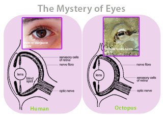
Figure 5 - The eye of a human and the eye of an octopus are nearly identical in structure, but evolved totally independently of each other. As Daniel Dennett pointed out, there are only a certain number of Good Tricks in Design Space and natural selection will drive different lines of descent towards them.

Figure 6 – There are many living fossils that have left behind signposts along the trail to the modern camera-like eye. Notice that the human-like eye on the far right is really that of an octopus (click to enlarge).
An excellent treatment of the significance that convergence has played in the evolutionary history of life on Earth, and possibly beyond, can be found in Life’s Solution (2003) by Simon Conway Morris. The convergent evolution for carbon-based life on the Earth to develop eyes was driven by the hardware fact of life that the Earth is awash in solar photons.
Programmers and living things both have to deal with the second law of thermodynamics and nonlinearity, and there are only a few optimal solutions. Programmers try new development techniques, and the successful techniques tend to survive and spread throughout the IT community, while the less successful techniques are slowly discarded. Over time, the population distribution of software techniques changes. As with the evolution of living things on Earth, the evolution of software has been greatly affected by the physical environment, or hardware, upon which it ran. Just as the Earth has not always been as it is today, the same goes for computing hardware. The evolution of software has been primarily affected by two things - CPU speed and memory size. As I mentioned in So You Want To Be A Computer Scientist?, the speed and memory size of computers have both increased by about a factor of a billion since Konrad Zuse built the Z3 in the spring of 1941, and the rapid advances in both and the dramatic drop in their costs have shaped the evolutionary history of software greatly. To fully understand those shaping forces of software evolution we must next explore the evolution of computer hardware.
A Brief Evolutionary History of Computer Hardware
It all started back in May of 1941 when Konrad Zuse first cranked up his Z3 computer. The Z3 was the world's first real computer and was built with 2400 electromechanical relays that were used to perform the switching operations that all computers use to store information and to process it. To build a computer, all you need is a large network of interconnected switches that have the ability to switch each other on and off in a coordinated manner. Switches can be in one of two states, either open (off) or closed (on), and we can use those two states to store the binary numbers of “0” or “1”. By using a number of switches teamed together in open (off) or closed (on) states, we can store even larger binary numbers, like “01100100” = 38. We can also group the switches into logic gates that perform logical operations. For example, in Figure 7 below we see an AND gate composed of two switches A and B. Both switch A and B must be closed in order for the light bulb to turn on. If either switch A or B is open, the light bulb will not light up.

Figure 7 – An AND gate can be simply formed from two switches. Both switches A and B must be closed, in a state of “1”, in order to turn the light bulb on.
Additional logic gates can be formed from other combinations of switches as shown in Figure 8 below. It takes about 2 - 8 switches to create each of the various logic gates shown below.
Figure 8 – Additional logic gates can be formed from other combinations of 2 – 8 switches.
Once you can store binary numbers with switches and perform logical operations upon them with logic gates, you can build a computer that performs calculations on numbers. To process text, like names and addresses, we simply associate each letter of the alphabet with a binary number, like in the ASCII code set where A = “01000001” and Z = ‘01011010’ and then process the associated binary numbers.

Figure 9 – Konrad Zuse with a reconstructed Z3 in 1961 (click to enlarge).

Figure 10 – Block diagram of the Z3 architecture (click to enlarge).
The electrical relays used by the Z3 were originally meant for switching telephone conversations. Closing one relay allowed current to flow to another relay’s coil, causing that relay to close as well.
Figure 11 – The Z3 was built using 2400 electrical relays, originally meant for switching telephone conversations.
Figure 12 – The electrical relays used by the Z3 for switching were very large, very slow and used a great deal of electricity which generated a great deal of waste heat.
To learn more about how Konrad Zuse built the world’s very first real computers - the Z1, Z2 and Z3 in the 1930s and early 1940s, see the following article that was written in his own words:
http://ei.cs.vt.edu/~history/Zuse.html
Now I was born about 10 years later in 1951, a few months after the United States government installed its very first commercial computer, a UNIVAC I, for the Census Bureau on June 14, 1951. The UNIVAC I was 25 feet by 50 feet in size and contained 5,600 vacuum tubes, 18,000 crystal diodes and 300 relays with a total memory of 12 K. From 1951 to 1958 a total of 46 UNIVAC I computers were built and installed.
Figure 13 – The UNIVAC I was very impressive on the outside.
Figure 14 – But the UNIVAC I was a little less impressive on the inside.
Figure 15 – Most of the electrical relays of the Z3 were replaced with vacuum tubes in the UNIVAC I, which were also very large, used lots of electricity and generated lots of waste heat too, but the vacuum tubes were 100,000 times faster than relays.
Figure 16 – Vacuum tubes contain a hot negative cathode that glows red and boils off electrons. The electrons are attracted to the cold positive anode plate, but there is a gate electrode between the cathode and anode plate. By changing the voltage on the grid, the vacuum tube can control the flow of electrons like the handle of a faucet. The grid voltage can be adjusted so that the electron flow is full blast, a trickle, or completely shut off, and that is how a vacuum tube can be used as a switch.
In the 1960s the vacuum tubes were replaced by discrete transistors and in the 1970s the discrete transistors were replaced by thousands of transistors on a single silicon chip. Over time, the number of transistors that could be put onto a silicon chip increased dramatically, and today, the silicon chips in your personal computer hold many billions of transistors that can be switched on and off in about 10-10 seconds. Now let us look at how these transistors work.
There are many different kinds of transistors, but I will focus on the FET (Field Effect Transistor) that is used in most silicon chips today. A FET transistor consists of a source, gate and a drain. The whole affair is laid down on a very pure silicon crystal using a multi-step process that relies upon photolithographic processes to engrave circuit elements upon the very pure silicon crystal. Silicon lies directly below carbon in the periodic table because both silicon and carbon have 4 electrons in their outer shell and are also missing 4 electrons. This makes silicon a semiconductor. Pure silicon is not very electrically conductive in its pure state, but by doping the silicon crystal with very small amounts of impurities, it is possible to create silicon that has a surplus of free electrons. This is called N-type silicon. Similarly, it is possible to dope silicon with small amounts of impurities that decrease the amount of free electrons, creating a positive or P-type silicon. To make an FET transistor you simply use a photolithographic process to create two N-type silicon regions onto a substrate of P-type silicon. Between the N-type regions is found a gate that controls the flow of electrons between the source and drain regions, like the grid in a vacuum tube. When a positive voltage is applied to the gate, it attracts the remaining free electrons in the P-type substrate and repels its positive holes. This creates a conductive channel between the source and drain which allows a current of electrons to flow.

Figure 17 – A FET transistor consists of a source, gate and drain. When a positive voltage is applied to the gate, a current of electrons can flow from the source to the drain and the FET acts like a closed switch that is “on”. When there is no positive voltage on the gate, no current can flow from the source to the drain, and the FET acts like an open switch that is “off”.
Figure 18 – When there is no positive voltage on the gate, the FET transistor is switched off, and when there is a positive voltage on the gate the FET transistor is switched on. These two states can be used to store a binary “0” or “1”, or can be used as a switch in a logic gate, just like an electrical relay or a vacuum tube.
Figure 19 – Above is a plumbing analogy that uses a faucet or valve handle to simulate the actions of the source, gate and drain of an FET transistor.
The CPU chip in your computer consists largely of transistors in logic gates, but your computer also has a number of memory chips that use transistors that are “on” or “off” and can be used to store binary numbers or text that is encoded using binary numbers. The next thing we need is a way to coordinate the billions of transistor switches in your computer. That is accomplished with a system clock. My current laptop has a clock speed of 2.5 GHz which means it ticks 2.5 billion times each second. Each time the system clock on my computer ticks, it allows all of the billions of transistor switches on my laptop to switch on, off, or stay the same in a coordinated fashion. So while your computer is running, it is actually turning on and off billions of transistors billions of times each second – and all for a few hundred dollars!
Computer memory was another factor greatly affecting the origin and evolution of software over time. Strangely, the original Z3 used electromechanical switches to store working memory, like we do today with transistors on memory chips, but that made computer memory very expensive and very limited, and this remained true all during the 1950s and 1960s. Prior to 1955 computers, like the UNIVAC I that first appeared in 1951, were using mercury delay lines that consisted of a tube of mercury that was about 3 inches long. Each mercury delay line could store about 18 bits of computer memory as sound waves that were continuously refreshed by quartz piezoelectric transducers on each end of the tube. Mercury delay lines were huge and very expensive per bit so computers like the UNIVAC I only had a memory of 12 K (98,304 bits).


Figure 20 – Prior to 1955, huge mercury delay lines built from tubes of mercury that were about 3 inches long were used to store bits of computer memory. A single mercury delay line could store about 18 bits of computer memory as a series of sound waves that were continuously refreshed by quartz piezoelectric transducers at each end of the tube.
In 1955 magnetic core memory came along, and used tiny magnetic rings called "cores" to store bits. Four little wires had to be threaded by hand through each little core in order to store a single bit, so although magnetic core memory was a lot cheaper and smaller than mercury delay lines, it was still very expensive and took up lots of space.
Figure 21 – Magnetic core memory arrived in 1955 and used a little ring of magnetic material, known as a core, to store a bit. Each little core had to be threaded by hand with 4 wires to store a single bit.
Figure 22 – Magnetic core memory was a big improvement over mercury delay lines, but it was still hugely expensive and took up a great deal of space within a computer.
Figure 23 – Finally in the early 1970s inexpensive semiconductor memory chips came along that made computer memory small and cheap.
Again, it was the relentless drive of software for ever-increasing amounts of memory and CPU-cycles that made all this happen, and that is why you can now comfortably sit in a theater with a smartphone that can store more than 64 billion bytes of data, while back in 1951 the UNIVAC I occupied an area of 25 feet by 50 feet to store 12,000 bytes of data. Like all forms of self-replicating information tend to do, over the past 2.5 billion seconds, software has opportunistically exapted the extant hardware of the day - the electromechanical relays, vacuum tubes, discrete transistors and transistor chips of the emerging telecommunications and consumer electronics industries, into the service of self-replicating software of ever-increasing complexity, as did carbon-based life exapt the extant organic molecules and the naturally occurring geochemical cycles of the day in order to bootstrap itself into existence.
But when I think back to my early childhood in the early 1950s, I can still vividly remember a time when there essentially was no software at all in the world. In fact, I can still remember my very first encounter with a computer on Monday, Nov. 19, 1956, watching the Art Linkletter TV show People Are Funny with my parents on an old black and white console television set that must have weighed close to 150 pounds. Art was showcasing the 21st UNIVAC I to be constructed and had it sorting through the questionnaires from 4,000 hopeful singles, looking for the ideal match. The machine paired up John Caran, 28, and Barbara Smith, 23, who later became engaged. And this was more than 40 years before eHarmony.com! To a five-year-old boy, a machine that could “think” was truly amazing. Since that very first encounter with a computer back in 1956, I have personally witnessed software slowly becoming the dominant form of self-replicating information on the planet, and I have also seen how software has totally reworked the surface of the planet to provide a secure and cozy home for more and more software of ever-increasing capability. For more on this please see A Brief History of Self-Replicating Information. That is why I think there would be much to be gained in exploring the origin and evolution of the $10 trillion computer simulation that the Software Universe provides, and that is what softwarephysics is all about. In the next sections, we will see how software converged upon the same solutions to fight the second law of thermodynamics and nonlinearity as did carbon-based life on the Earth. But first a little more geology.
The Coevolution of Carbon-Based Life and the Earth's Crust
In the above section, we saw that the two fundamental factors influencing the evolution of computer hardware were the nature and speed of switches and the nature and capacity of computer memory. In the sections that follow, we will see that these two fundamental hardware factors also greatly influenced the evolution of software over the past 2.5 billion seconds. And the demands made by the ever-increasing levels of software complexity over time also drove the evolution of faster computers with much more memory in a similar fashion to the coevolution that we saw between carbon-based life and the rocks of the Earth's crust.
The two major environmental factors affecting the evolution of living things on Earth have been the amount of solar energy arriving from the Sun and the atmospheric gases surrounding the Earth that held it in. The size and distribution of the Earth’s continents and oceans have also had an influence on the Earth’s overall environmental characteristics too, as the continents shuffled around the surface of the Earth, responding to the forces of plate tectonics. For example, billions of years ago the Sun was actually less bright than it is today. Our Sun is a star on the main sequence that is using the proton-proton reaction and the carbon-nitrogen-oxygen cycle in its core to turn hydrogen into helium-4, and consequently, turn matter into energy that is later radiated away from its surface, ultimately reaching the Earth. As a main-sequence star ages, it begins to shift from the proton-proton reaction to relying more on the carbon-nitrogen-oxygen cycle which runs at a higher temperature. Thus, as a main-sequence star ages, its core heats up and it begins to radiate more energy at its surface. In fact, the Sun currently radiates about 30% more energy today than it did about 4.5 billion years ago when it first formed and entered the main sequence. Over the past billion years, the Sun has been getting about 1% brighter each 100 million years. But this increase in the Sun’s radiance has been offset by a corresponding drop in greenhouse gases, like carbon dioxide, over this same period of time, otherwise, the Earth’s oceans would have vaporized long ago, and the Earth would now have a climate more like Venus which has a surface temperature that melts lead. Using some simple physics, you can quickly calculate that if the Earth did not have an atmosphere containing greenhouse gases like carbon dioxide, the surface of the Earth would be on average 600F cooler today and totally covered by ice. Thankfully there has been a long-term decrease in the amount of carbon dioxide in the Earth’s atmosphere, principally caused by living things extracting carbon dioxide from the air to make carbon-based molecules. These carbon-based molecules later get deposited into sedimentary rocks which plunge back into the Earth at the many subduction zones around the world that result from plate tectonic activities. For example, hundreds of millions of years ago, the Earth’s atmosphere contained about 10 - 20 times as much carbon dioxide as it does today and held in more heat from the dimmer Sun. So greenhouse gases like carbon dioxide have played a critical role in keeping the Earth’s climate in balance and suitable for life.
The third factor that has greatly affected the course of evolution on Earth has been the occurrence of periodic mass extinctions. In 1860, John Philips, an English geologist, recognized three major geological eras based upon dramatic changes in fossils brought about by two mass extinctions. He called the eras the Paleozoic (Old Life), the Mesozoic (Middle Life), and the Cenozoic (New Life), defined by mass extinctions at the Paleozoic-Mesozoic and Mesozoic-Cenozoic boundaries:
Cenozoic 65 my – present
=================== <= Mass Extinction
Mesozoic 250 my – 65 my
=================== <= Mass Extinction
Paleozoic 541 my – 250 my
Of course, John Philips knew nothing of radiometric dating in 1860, so these geological eras only provided for a means of relative dating of rock strata based upon fossil content. The absolute date ranges only came later in the 20th century, with the advent of radiometric dating of volcanic rock layers found between the layers of fossil-bearing sedimentary rock. It is now known that we have actually had five major mass extinctions since multicellular life first began to flourish about 541 million years ago, and there have been several lesser extinction events as well. The three geological eras have been further subdivided into geological periods, like the Cambrian at the base of the Paleozoic, the Permian at the top of the Paleozoic, the Triassic at the base of the Mesozoic, and the Cretaceous at the top of the Mesozoic. Figure 24 shows an “Expand All” of the current geological time scale now in use. Notice how small the Phanerozoic is, the eon comprising the Paleozoic, Mesozoic, and Cenozoic eras in which complex plant and animal life are found. Indeed, the Phanerozoic represents only the last 12% of the Earth’s history – the first 88% of the Earth’s history was dominated by simple single-celled forms of life like bacteria.

Figure 24 - The Geological Time Scale of the Phanerozoic Eon is divided into the Paleozoic, Mesozoic and Cenozoic Eras by two great mass extinctions - click to enlarge.
Figure 25 - Life in the Paleozoic, before the Permian-Triassic mass extinction, was far different than life in the Mesozoic.
Figure 26 - In the Mesozoic the dinosaurs ruled after the Permian-Triassic mass extinction, but small mammals were also present.
Figure 27 - Life in the Cenozoic, following the Cretaceous-Tertiary mass extinction, has so far been dominated by the mammals. This will likely soon change as software becomes the dominant form of self-replicating information on the planet, ushering in a new geological Era that has yet to be named.
Currently, it is thought that these mass extinctions arise from two different sources. One type of mass extinction is caused by the impact of a large comet or asteroid and has become familiar to the general public as the Cretaceous-Tertiary (K-T) mass extinction that wiped out the dinosaurs at the Mesozoic-Cenozoic boundary 65 million years ago. An impacting mass extinction is characterized by a rapid extinction of species followed by a corresponding rapid recovery in a matter of a few million years. An impacting mass extinction is like turning off a light switch. Up until the day the impactor hits the Earth, everything is fine and the Earth has a rich biosphere. After the impactor hits the Earth, the light switch turns off and there is a dramatic loss of species diversity. However, the effects of the incoming comet or asteroid are geologically brief and the Earth’s environment returns to normal in a few decades or less, so within a few million years or so, new species rapidly evolve to replace those that were lost.
The other kind of mass extinction is thought to arise from an overabundance of greenhouse gases and a dramatic drop in oxygen levels and is typified by the Permian-Triassic (P-T) mass extinction at the Paleozoic-Mesozoic boundary 250 million years ago. Greenhouse extinctions are thought to be caused by periodic flood basalts, like the Siberian Traps flood basalt of the late Permian. A flood basalt begins as a huge plume of magma several hundred miles below the surface of the Earth. The plume slowly rises and eventually breaks the surface of the Earth, forming a huge flood basalt that spills basaltic lava over an area of millions of square miles to a depth of several thousand feet. Huge quantities of carbon dioxide bubble out of the magma over a period of several hundreds of thousands of years and greatly increase the ability of the Earth’s atmosphere to trap heat from the Sun. For example, during the Permian-Triassic mass extinction, carbon dioxide levels may have reached a level as high as 3,000 ppm, much higher than the current 410 ppm. Most of the Earth warms to tropical levels with little temperature difference between the equator and the poles. This shuts down the thermohaline conveyor that drives the ocean currents. Currently, the thermohaline conveyor begins in the North Atlantic, where high winds and cold polar air reduce the temperature of ocean water through evaporation and concentrates its salinity, making the water very dense. The dense North Atlantic water, with lots of dissolved oxygen, then descends to the ocean depths and slowly winds its way around the entire Earth, until it ends up back on the surface in the North Atlantic several thousand years later. When this thermohaline conveyor stops for an extended period of time, the water at the bottom of the oceans is no longer supplied with oxygen, and only bacteria that can survive on sulfur compounds manage to survive in the anoxic conditions. These sulfur-loving bacteria metabolize sulfur compounds to produce large quantities of highly toxic hydrogen sulfide gas, the distinctive component of the highly repulsive odor of rotten eggs, which has a severely damaging effect on both marine and terrestrial species. The hydrogen sulfide gas also erodes the ozone layer by dropping oxygen levels down to a suffocating low of 12% of the atmosphere, compared to the current level of 21%, allowing damaging ultraviolet light to reach the Earth’s surface, and to beat down relentlessly upon the animal life gasping for breath in an oxygen-poor atmosphere even at sea level and destroy its DNA. . The combination of severe climate change, changes to atmospheric and oceanic oxygen levels and temperatures, the toxic effects of hydrogen sulfide gas, and the loss of the ozone layer, cause a slow extinction of many species over a period of several hundred thousand years. And unlike an impacting mass extinction, a greenhouse gas mass extinction does not quickly reverse itself but persists for millions of years until the high levels of carbon dioxide are flushed from the atmosphere and oxygen levels rise. In the stratigraphic section, this is seen as a thick section of rock with decreasing numbers of fossils and fossil diversity leading up to the mass extinction, and a thick layer of rock above the mass extinction level with very few fossils at all, representing the long recovery period of millions of years required to return the Earth’s environment back to a more normal state. There are a few good books by Peter Ward that describe these mass extinctions more fully, The Life and Death of Planet Earth (2003), Gorgon – Paleontology, Obsession, and the Greatest Catastrophe in Earth’s History (2004), and Out of Thin Air (2006). There is also the disturbing Under a Green Sky (2007), which posits that we might be initiating a human-induced greenhouse gas mass extinction by burning up all the fossil fuels that have been laid down over hundreds of millions of years in the Earth’s strata. For a deep-dive into the Permian-Triassic mass extinction, see Professor Benjamin Burger's excellent YouTube at:
The Permian-Triassic Boundary - The Rocks of Utah
https://www.youtube.com/watch?v=uDH05Pgpel4&list=PL9o6KRlci4eD0xeEgcIUKjoCYUgOvtpSo&t=1s
The above video is just over an hour in length, and it shows Professor Burger collecting rock samples at the Permian-Triassic Boundary in Utah and then performing lithological analyses of them in the field. He then brings the samples to his lab for extensive geochemical analysis. This YouTube provides a rare opportunity for nonprofessionals to see how actual geological fieldwork and research are performed. You can also view a pre-print of the scientific paper that he has submitted to the journal Global and Planetary Change at:
What caused Earth’s largest mass extinction event?
New evidence from the Permian-Triassic boundary in northeastern Utah
https://eartharxiv.org/khd9y
In How to Use Your IT Skills to Save the World and Last Call for Carbon-Based Intelligence on Planet Earth I explained how you could help to avoid this disaster.

Figure 28 - Above is a map showing the extent of the Siberian Traps flood basalt. The above area was covered by flows of basaltic lava to a depth of several thousand feet.
Figure 29 - Here is an outcrop of the Siberian Traps formation. Notice the sequence of layers. Each new layer represents a massive outflow of basaltic lava that brought greenhouse gases to the surface.
Over the past 40 years, there has been a paradigm shift in paleontology beginning with the discovery in 1980 by Luis Alvarez of a thin layer of iridium-rich clay at the Cretaceous-Tertiary (K-T) mass extinction boundary, which has been confirmed in deposits throughout the world. This discovery, along with the presence of shocked quartz grains in these same layers, convinced the paleontological community that the K-T mass extinction was the result of an asteroid or comet strike upon the Earth. Prior to the Alvarez discovery, most paleontologists thought that mass extinctions resulted from slow environmental changes that occurred over many millions of years. Similarly, within the past 10 years, there has been a similar shift in thinking for the mass extinctions that are not caused by impactors. Rather than ramping up over many millions of years, the greenhouse gas mass extinctions seem to unfold in a few hundred thousand years or less, which is a snap of the fingers in geological Deep Time.
In James Hutton’s Theory of the Earth (1785) and Charles Lyell’s Principles of Geology (1830), the principle of uniformitarianism was laid down in the early 19th century. Uniformitarianism is a geological principle that states that the “present is key to the past”. If you want to figure out how a 100 million-year-old cross-bedded sandstone came to be, just dig into a point bar on a modern-day river or into a wind-blown sand dune and take a look.

Figure 30 – The cross-bedding found when digging into a modern sand dune explains how the cross-bedding in ancient sandstones came to be.
Figure 31 – Cross-bedding in sandstones arises when sand is pushed by a fluid, such as wind or water. The cross-bedding tells you which way was "up" when the sandstone was deposited and which way the fluid was flowing too.
Uniformitarianism contends that the Earth has been shaped by slow-acting geological processes that can still be observed at work today. Uniformitarianism replaced the catastrophism of the 18th century which proposed that the geological structures of the Earth were caused by short-term catastrophic events like Noah’s flood. In fact, the names for the Tertiary and Quaternary geological periods actually come from those days! In the 18th century, it was thought that the water from Noah’s flood receded in four stages - Primary, Secondary, Tertiary and Quaternary, and each stage laid down different kinds of rock as it withdrew. Now since most paleontologists are really geologists who have specialized in studying fossils, the idea of uniformitarianism unconsciously crept into paleontology as well. Because uniformitarianism proposed that the rock formations of the Earth slowly changed over immense periods of time, so too must the Earth’s biosphere have slowly changed over long periods of time, and therefore, the mass extinctions must have been caused by slow-acting environmental changes occurring over many millions of years.
But now we have come full circle. Yes, uniformitarianism may be very good for describing the slow evolution of hard-as-nails rocks, but maybe not so good for the evolution of squishy living things that are much more sensitive to things like asteroid strikes or greenhouse gas emissions that mess with the Earth’s climate over geologically brief periods of time. Uniformitarianism may be the general rule for the biosphere, as Darwin’s mechanisms of inheritance, innovation and natural selection slowly work upon the creatures of the Earth. But every 100 million years or so, something goes dreadfully wrong with the Earth’s climate and environment, and Darwin’s process of natural selection comes down hard upon the entire biosphere, winnowing out perhaps 70% - 90% of the species on Earth that cannot deal with the new geologically temporary conditions. This causes dramatic evolutionary effects. For example, the Permian-Triassic (P-T) mass extinction cleared the way for the surviving reptiles to evolve into the dinosaurs that ruled the Mesozoic, and the Cretaceous-Tertiary (K-T) mass extinction, did the same for the rodent-like mammals that went on to conquer the Cenozoic, ultimately producing a species capable of producing software.
The Evolution of Software Over the Past 2.5 Billion Seconds Has Also Been Heavily Influenced by Mass Extinctions
Similarly, IT experienced a similar devastating mass extinction during the early 1990s when we experienced an environmental change that took us from the Age of the Mainframes to the Distributed Computing Platform. Suddenly mainframe Cobol/CICS and Cobol/DB2 programmers were no longer in demand. Instead, everybody wanted C and C++ programmers who worked on cheap Unix servers. This was a very traumatic time for IT professionals. Of course, the mainframe programmers never went entirely extinct, but their numbers were greatly reduced. The number of IT workers in mainframe Operations also dramatically decreased, while at the same time the demand for Operations people familiar with the Unix-based software of the new Distributed Computing Platform skyrocketed. This was around 1992, and at the time I was a mainframe programmer used to working with IBM's MVS and VM/CMS operating systems, writing Cobol, PL-1 and REXX code using DB2 databases. So I had to teach myself Unix and C and C++ to survive. In order to do that, I bought my very first PC, an 80-386 machine running Windows 3.0 with 5 MB of memory and a 100 MB hard disk for $1500. I also bought the Microsoft C7 C/C++ compiler for something like $300. And that was in 1992 dollars! One reason for the added expense was that there were no Internet downloads in those days because there were no high-speed ISPs. PCs did not have CD/DVD drives either, so the software came on 33 diskettes, each with a 1.44 MB capacity, that had to be loaded one diskette at a time in sequence. The software also came with about a foot of manuals describing the C++ class library on very thin paper. Indeed, suddenly finding yourself to be obsolete is not a pleasant thing and calls for drastic action.

Figure 32 – An IBM OS/360 mainframe from 1964. The IBM OS/360 mainframe caused commercial software to explode within corporations and gave IT professionals the hardware platform that they were waiting for.
Figure 33 – The Distributed Computing Platform replaced a great deal of mainframe computing with a large number of cheap self-contained servers running software that tied the servers together.
The problem with the Distributed Computing Platform was that although the server hardware was cheaper than mainframe hardware, the granular nature of the Distributed Computing Platform meant that it created a very labor-intensive infrastructure that was difficult to operate and support, and as the level of Internet traffic dramatically expanded over the past 20 years, the Distributed Computing Platform became nearly impossible to support. For example, I worked in Middleware Operations for the Discover credit card company from 2002 - 2016, and during that time our Distributed Computing Platform infrastructure exploded by a factor of at least a hundred. It finally became so complex and convoluted that we could barely keep it all running, and we really did not even have enough change window time to properly apply maintenance to it as I described in The Limitations of Darwinian Systems. Clearly, the Distributed Computing Platform was not sustainable, and an alternative was desperately needed. This is because the Distributed Computing Platform was IT's first shot at running software on a multicellular architecture, as I described in Software Embryogenesis. But the Distributed Computing Platform simply had too many moving parts, all working together independently on their own, to fully embrace the advantages of a multicellular organization. In many ways, the Distributed Computing Platform was much like the ancient stromatolites that tried to reap the advantages of a multicellular organism by simply tying together the diverse interests of multiple layers of prokaryotic cyanobacteria into a "multicellular organism" that seemingly benefited the interests of all.

Figure 34 – Stromatolites are still found today in Sharks Bay Australia. They consist of mounds of alternating layers of prokaryotic bacteria.
Figure 35 – The cross-section of an ancient stromatolite displays the multiple layers of prokaryotic cyanobacteria that came together for their own mutual self-survival to form a primitive "multicellular" organism that seemingly benefited the interests of all. The servers and software of the Distributed Computing Platform were very much like the primitive stromatolites.
The collapse of the Distributed Computing Platform under its own weight brought on a second mass extinction beginning in 2010 with the rise of Cloud Computing.
The Rise of Cloud Computing Causes the Second Great Software Mass Extinction
The successor architecture to the Distributed Computing Platform was the Cloud Computing Platform, which is usually displayed as a series of services all stacked into levels. The highest level, SaaS (Software as a Service) runs the common third-party office software like Microsoft Office 365 and email. The second level, PaaS (Platform as a Service) is where the custom business software resides, and the lowest level, IaaS (Infrastructure as a Service) provides for an abstract tier of virtual servers and other resources that automatically scale with varying load levels. From an Applications Development standpoint, the PaaS layer is the most interesting because that is where they will be installing the custom application software used to run the business and also to run high-volume corporate websites that their customers use. Currently, that custom application software is installed into the middleware that is running on the Unix servers of the Distributed Computing Platform. The PaaS level will be replacing the middleware software, such as the Apache webservers and the J2EE Application servers, like WebSphere, Weblogic and JBoss that currently do that. For Operations, the IaaS level, and to a large extent, the PaaS level too are of most interest because those levels will be replacing the middleware and other support software running on hundreds or thousands of individual self-contained servers. The Cloud architecture can be run on a company's own hardware, or it can be run on a timesharing basis on the hardware at Amazon, Microsoft, IBM or other Cloud providers, using the Cloud software that the Cloud providers market.

Figure 36 – Cloud Computing returns us to the timesharing days of the 1960s and 1970s by viewing everything as a service.
Basically, the Cloud Computing Platform is based on two defining characteristics:
1. Returning to the timesharing days of the 1960s and 1970s when many organizations could not afford to support a mainframe infrastructure of their own.
2. Taking the multicellular architecture of the Distributed Computing Platform to the next level by using Cloud Platform software to produce a full-blown multicellular organism, and even higher, by introducing the self-organizing behaviors of the social insects like ants and bees.
For more on this see Cloud Computing and the Coming Software Mass Extinction and The Origin and Evolution of Cloud Computing - Software Moves From the Sea to the Land and Back Again.
The Geological Time Scale of Software Evolution
Similarly, the evolutionary history of software over the past 2.5 billion seconds has also been greatly affected by a series of mass extinctions, which allow us to also subdivide the evolutionary history of software into several long computing eras, like the geological eras listed above. As with the evolution of the biosphere over the past 541 million years, we shall see that these mass extinctions of software have also been caused by several catastrophic events in IT that were separated by long periods of slow software evolution through uniformitarianism. Like the evolution of carbon-based life on the Earth, some of these software mass extinctions were caused by some drastic environmental hardware changes, while others were simply caused by drastic changes in the philosophy of software development thought.
Unstructured Period (1941 – 1972)
During the Unstructured Period, programs were simple monolithic structures with lots of GOTO statements, no subroutines, no indentation of code, and very few comment statements. The machine code programs of the 1940s evolved into the assembler programs of the 1950s and the compiled programs of the 1960s, with FORTRAN appearing in 1956 and COBOL in 1958. These programs were very similar to the early prokaryotic bacteria that appeared over 4,000 million years ago on Earth and lacked internal structure. Bacteria essentially consist of a tough outer cell wall enclosing an inner cell membrane and contain a minimum of internal structure. The cell wall is composed of a tough molecule called peptidoglycan, which is composed of tightly bound amino sugars and amino acids. The cell membrane is composed of phospholipids and proteins, which will be described later in this posting. The DNA within bacteria generally floats freely as a large loop of DNA, and their ribosomes, used to help transcribe DNA into proteins, float freely as well and are not attached to membranes called the rough endoplasmic reticulum. The chief advantage of bacteria is their simple design and ability to thrive and rapidly reproduce even in very challenging environments, like little AK-47s that still manage to work in environments where modern tanks fail. Just as bacteria still flourish today, some unstructured programs are still in production.

Figure 37 – A simple prokaryotic bacterium with little internal structure (click to enlarge)
Below is a code snippet from a fossil FORTRAN program listed in a book published in 1969 showing little internal structure. Notice the use of GOTO statements to skip around in the code. Later this would become known as the infamous “spaghetti code” of the Unstructured Period that was such a joy to support.
30 DO 50 I=1,NPTS
31 IF (MODE) 32, 37, 39
32 IF (Y(I)) 35, 37, 33
33 WEIGHT(I) = 1. / Y(I)
GO TO 41
35 WEIGHT(I) = 1. / (-1*Y(I))
37 WEIGHT(I) = 1.
GO TO 41
39 WEIGHT(I) = 1. / SIGMA(I)**2
41 SUM = SUM + WEIGHT(I)
YMEAN = WEIGHT(I) * FCTN(X, I, J, M)
DO 44 J = 1, NTERMS
44 XMEAN(J) = XMEAN(J) + WEIGHT(I) * FCTN(X, I, J, M)
50 CONTINUE
The primitive nature of software in the Unstructured Period was largely due to the primitive nature of the hardware upon which it ran. Figure 43 shows an IBM OS/360 from 1964 – notice the operator at the teletype feeding commands to the nearby operator console, the distant tape drives, and the punch card reader in the mid-ground. Such a machine had about 1 MB of memory, less than 1/1000 of the memory of a current cheap $250 PC, and a matching anemic processing speed. For non-IT readers let me remind all that:
1 KB = 1 kilobyte = 210 = 1024 bytes or about 1,000 bytes
1 MB = 1 megabyte = 1024 x 1024 = 1,048,576 bytes or about a million bytes
1 GB = 1 gigabyte = 1024 x 10224 x 1024 = 1,073,741,824 bytes or about a billion bytes
One byte of memory can store one ASCII text character like an “A” and two bytes can store a small integer in the range of -32,768 to +32,767. When I first started programming in 1972 we thought in terms of kilobytes, then megabytes, and now gigabytes. Data science people now think in terms of many terabytes - 1 TB = 1024 GB.
Software was input via punched cards and the output was printed on fan-fold paper. Compiled code could be stored on tape or very expensive disk drives if you could afford them, but any changes to code were always made via punched cards, and because you were only allowed perhaps 128K – 256K of memory for your job, programs had to be relatively small, so simple unstructured code ruled the day. Like the life cycle of a single-celled bacterium, the compiled and linked code for your program was loaded into the memory of the computer at execution time and did its thing in a batch mode, until it completed successfully or abended and died. At the end of the run, the computer’s memory was released for the next program to be run and your program ceased to exist.
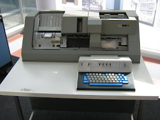
Figure 38 - An IBM 029 keypunch machine from the 1960s Unstructured Period of software.

Figure 39 - Each card could hold a maximum of 80 bytes. Normally, one line of code was punched onto each card.
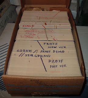
Figure 40 - The cards for a program were held together into a deck with a rubber band, or for very large programs, the deck was held in a special cardboard box that originally housed blank cards. Many times the data cards for a run followed the cards containing the source code for a program. The program was compiled and linked in two steps of the run and then the generated executable file processed the data cards that followed in the deck.
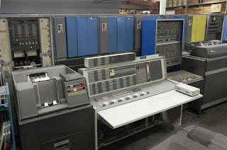
Figure 41 - To run a job, the cards in a deck were fed into a card reader, as shown on the left above, to be compiled, linked, and executed by a million-dollar mainframe computer. In the above figure, the mainframe is located directly behind the card reader.
Figure 42 - The output of programs was printed on fan-folded paper by a line printer.
However, one should not discount the great advances that were made by the early bacteria billions of years ago or by the unstructured code from the computer systems of the 1950s and 1960s. These were both very important formative periods in the evolution of life and of software on Earth, and examples of both can still be found in great quantities today. For example, it is estimated that about 50% of the Earth’s biomass is still composed of simple bacteria. Your body consists of about 100 trillion cells, but you also harbor about 10 times that number of bacterial cells that are in a parasitic/symbiotic relationship with the “other” cells of your body and perform many of the necessary biochemical functions required to keep you alive, such as aiding with the digestion of food. Your gut contains about 3.5 pounds of active bacteria and about 50% of the dry weight of your feces is bacteria, so in reality, we are all composed of about 90% bacteria with only 10% of our cells being “normal” human cells.
All of the fundamental biochemical pathways used by living things to create large complex organic molecules from smaller monomers, or to break those large organic molecules back down into simple monomers were first developed by bacteria billions of years ago. For example, bacteria were the first forms of life to develop the biochemical pathways that turn carbon dioxide, water, and the nitrogen in the air into the organic molecules necessary for life – sugars, lipids, amino acids, and the nucleotides that form RNA and DNA. They also developed the biochemical pathways to replicate DNA and transcribe DNA into proteins, and to form complex structures such as cell walls and cell membranes from sugars, amino acids, proteins, and phospholipids. Additionally, bacteria invented the Krebs cycle to break these large macromolecules back down to monomers for reuse and to release and store energy by transforming ADP to ATP. To expand upon this, we will see in Software Symbiogenesis, how Lynn Margulis has proposed that all the innovations of large macroscopic forms of life have actually been acquired from the highly productive experiments of bacterial life forms.
Similarly, all of the fundamental coding techniques of IT at the line of code level were first developed in the Unstructured Period of the 1950s and 1960s, such as the use of complex variable names, arrays, nested loops, loop counters, if-then-else logic, list processing with pointers, I/O blocking, bubble sorts, etc. When I was in Middleware Operations for Discover, I did not do much coding. However, I did write a large number of Unix shell scripts to help make my job easier. These Unix shell scripts were small unstructured programs in the range of 10 – 50 lines of code, and although they were quite primitive and easy to write, they had a huge economic pay-off for me. Many times, a simple 20 line Unix shell script that took less than an hour to write, would provide as much value to me as the code behind the IBM Websphere Console, which I imagine probably had cost IBM about $10 - $100 million dollars to develop and came to several hundred thousand lines of code. For more on that see
MISE in the Attic. So if you add up all the little unstructured Unix shell scripts, DOS .bat files, edit macros, Excel spreadsheet macros, Word macros, etc., I bet that at least 50% of the software in the Software Universe is still unstructured code.
Figure 43 – An IBM OS/360 mainframe from 1964. The IBM OS/360 mainframe caused commercial software to explode within corporations during the Unstructured Period and gave IT professionals the hardware platform that they were waiting for.
Structured Period (1972 – 1992)
The increasing availability of computers with more memory and faster CPUs allowed for much larger programs to be written in the 1970s, but unstructured code became much harder to maintain as it grew in size, so the need for internal structure became readily apparent. Plus, around this time code began to be entered via terminals using full-screen editors, rather than on punched cards, which made it easier to view larger sections of code as you changed it.
Figure 44 - IBM 3278 terminals were connected to controllers that connected to IBM mainframes The IBM 3278 terminals then ran interactive TSO sessions with the IBM mainframes. The ISPF full-screen editor was then brought up under TSO after you logged into a TSO session.

Figure 45 – A mainframe with IBM 3278 CRT terminals attached (click to enlarge)
In 1972, Dahl, Dijkstra, and Hoare published Structured Programming, in which they suggested that computer programs should have complex internal structure with no GOTO statements, lots of subroutines, indented code, and many comment statements. During the Structured Period, these structured programming techniques were adopted by the IT community, and the GOTO statements were replaced by subroutines, also known as functions(), and indented code with lots of internal structure, like the eukaryotic structure of modern cells that appeared about 1,500 million years ago. Eukaryotic cells are found in the bodies of all complex organisms from single-cell yeasts to you and me and divide up cell functions amongst a collection of organelles (subroutines), such as mitochondria, chloroplasts, Golgi bodies, and the endoplasmic reticulum.

Figure 46 – Plants and animals are composed of eukaryotic cells with much internal structure (click to enlarge)
Figure 47 compares the simple internal structure of a typical prokaryotic bacterium with the internal structure of eukaryotic plant and animal cells. These eukaryotic cells could be simple single-celled plants and animals or they could be found within a much larger multicellular organism consisting of trillions of eukaryotic cells. Figure 47 is a bit deceiving, in that eukaryotic cells are huge cells that are more than 20 times larger in diameter than a typical prokaryotic bacterium with about 10,000 times the volume as shown in Figure 48. Because eukaryotic cells are so large, they have an internal cytoskeleton, composed of linear-shaped proteins that form filaments that act like a collection of tent poles, to hold up the huge cell membrane encircling the cell.
Eukaryotic cells also have a great deal of internal structure, in the form of organelles, that are enclosed by internal cell membranes. Like the structured programs of the 1970s and 1980s, eukaryotic cells divide up functions amongst these organelles. These organelles include the nucleus to store and process the genes stored in DNA, mitochondria to perform the Krebs cycle to create ATP from carbohydrates, and chloroplasts in plants to produce energy-rich carbohydrates from water, carbon dioxide, and sunlight.

Figure 47 – The prokaryotic cell architecture of the bacteria and archaea is very simple and designed for rapid replication. Prokaryotic cells do not have a nucleus enclosing their DNA. Eukaryotic cells, on the other hand, store their DNA on chromosomes that are isolated in a cellular nucleus. Eukaryotic cells also have a very complex internal structure with a large number of organelles, or subroutine functions, that compartmentalize the functions of life within the eukaryotic cells.
Figure 48 – Not only are eukaryotic cells much more complicated than prokaryotic cells, but they are also HUGE!
The introduction of structured programming techniques in the early 1970s allowed programs to become much larger and much more complex by using many subroutines to divide up logic into self-contained organelles. This induced a mass extinction of unstructured programs, similar to the Permian-Triassic (P-T) mass extinction, or the Great Dying, 250 million years ago that divided the Paleozoic from the Mesozoic in the stratigraphic column and resulted in the extinction of about 90% of the species on Earth. As programmers began to write new code using the new structured programming paradigm, older code that was too difficult to rewrite in a structured manner remained as legacy “spaghetti code” that slowly fossilized over time in production. Like the Permian-Triassic (P-T) mass extinction, the mass extinction of unstructured code in the 1970s was more like a greenhouse gas mass extinction than an impactor mass extinction because it spanned nearly an entire decade, and was also a rather complete mass extinction which totally wiped out most unstructured code in corporate systems.
Below is a code snippet from a fossil COBOL program listed in a book published in 1975. Notice the structured programming use of indented code and calls to subroutines with PERFORM statements.
PROCEDURE DIVISION.
OPEN INPUT FILE-1, FILE-2
PERFORM READ-FILE-1-RTN.
PERFORM READ-FILE-2-RTN.
PERFORM MATCH-CHECK UNTIL ACCT-NO OF REC-1 = HIGH_VALUES.
CLOSE FILE-1, FILE-2.
MATCH-CHECK.
IF ACCT-NO OF REC-1 < ACCT-NO OF REC-2
PERFORM READ-FILE-1-RTN
ELSE
IF ACCT-NO OF REC-1 > ACCT-NO OF REC-2
DISPLAY REC-2, 'NO MATCHING ACCT-NO'
PERORM READ-FILE-1-RTN
ELSE
PERORM READ-FILE-2-RTN UNTIL ACCT-NO OF REC-1
NOT EQUAL TO ACCT-NO OF REC-2
When I encountered my very first structured FORTRAN program in 1975, I diligently “fixed” the program by removing all the code indentations! You see in those days, we rarely saw the entire program on a line printer listing because that took a compile of the program to produce and wasted valuable computer time, which was quite expensive back then. When I provided an estimate for a new system back then, I figured 25% for programming manpower, 25% for overhead charges from other IT groups on the project, and 50% for compiles. So instead of working with a listing of the program, we generally flipped through the card deck of the program to do debugging. Viewing indented code in a card deck can give you a real headache, so I just “fixed” the program by making sure all the code started in column 7 of the punch cards as it should!
Object-Oriented Period (1992 – Present)
During the Object-Oriented Period, programmers adopted a multicellular organization for software, in which programs consisted of many instances of objects (cells) that were surrounded by membranes studded with exposed methods (membrane receptors).
The following discussion might be a little hard to follow for readers with a biological background, but with little IT experience, so let me define a few key concepts with their biological equivalents.
Class – Think of a class as a cell type. For example, the class Customer is a class that defines the cell type of Customer and describes how to store and manipulate the data for a Customer, like firstName, lastName, address, and accountBalance. For example, a program might instantiate a Customer object called “steveJohnston”.
Object – Think of an object as a cell. A particular object will be an instance of a class. For example, the object steveJohnston might be an instance of the class Customer and will contain all the information about my particular account with a corporation. At any given time, there could be many millions of Customer objects bouncing around in the IT infrastructure of a major corporation’s website.
Instance – An instance is a particular object of a class. For example, the steveJohnston object would be a particular instance of the class Customer, just as a particular red blood cell would be a particular instance of the cell type RedBloodCell. Many times programmers will say things like “This instantiates the Customer class”, meaning it creates objects (cells) of the Customer class (cell type).
Method – Think of a method() as a biochemical pathway. It is a series of programming steps or “lines of code” that produce a macroscopic change in the state of an object (cell). The Class for each type of object defines the data for the class, like firstName, lastName, address, and accountBalance, but it also defines the methods() that operate upon these data elements. Some methods() are public, while others are private. A public method() is like a receptor on the cell membrane of an object (cell). Other objects(cells) can send a message to the public methods of an object (cell) to cause it to execute a biochemical pathway within the object (cell). For example, steveJohnston.setFirstName(“Steve”) would send a message to the steveJohnston object instance (cell) of the Customer class (cell type) to have it execute the setFirstName method() to change the firstName of the object to “Steve”. The steveJohnston.getaccountBalance() method would return my current account balance with the corporation. Objects also have many internal private methods() within that are biochemical pathways that are not exposed to the outside world. For example, the calculateAccountBalance() method could be an internal method that adds up all of my debits and credits and updates the accountBalance data element within the steveJohnston object, but this method cannot be called by other objects (cells) outside of the steveJohnston object (cell). External objects (cells) have to call the steveJohnston.getaccountBalance() in order to find out my accountBalance.
Line of Code – This is a single statement in a method() like:
discountedTotalCost = (totalHours * ratePerHour) - costOfNormalOffset;
Remember methods() are the equivalent of biochemical pathways and are composed of many lines of code, so each line of code is like a single step in a biochemical pathway. Similarly, each character in a line of code can be thought of as an atom, and each variable as an organic molecule. Each character can be in one of 256 ASCII quantum states defined by 8 quantized bits, with each bit in one of two quantum states “1” or “0”, which can also be characterized as 8 electrons in a spin-up ↑ or spin-down ↓ state:
discountedTotalCost = (totalHours * ratePerHour) - costOfNormalOffset;
C = 01000011 = ↓ ↑ ↓ ↓ ↓ ↓ ↑ ↑
H = 01001000 = ↓ ↑ ↓ ↓ ↑ ↓ ↓ ↓
N = 01001110 = ↓ ↑ ↓ ↓ ↑ ↑ ↑ ↓
O = 01001111 = ↓ ↑ ↓ ↓ ↑ ↑ ↑ ↑
Programmers have to assemble characters (atoms) into organic molecules (variables) to form the lines of code that define a method() (biochemical pathway). As in carbon-based biology, the slightest error in a method() can cause drastic and usually fatal consequences. Because there is nearly an infinite number of ways of writing code incorrectly and only a very few ways of writing code correctly, there is an equivalent of the second law of thermodynamics at work. This simulated second law of thermodynamics and the very nonlinear macroscopic effects that arise from small coding errors is why software architecture has converged upon Life’s Solution. With these concepts in place, we can now proceed with our comparison of the evolution of software and carbon-based life on Earth.
Object-oriented programming actually started in the 1960s with Simula, the first language to use the concept of merging data and functions into objects defined by classes, but object-oriented programming did not really catch on until nearly 30 years later:
1962 - 1965 Dahl and Nygaard develop the Simula language
1972 - Smalltalk language developed
1983 - 1985 Sroustrup develops C++
1995 - Sun announces Java at SunWorld `95
Similarly, multicellular organisms first appeared about 900 million years ago, but it took about another 400 million years, until the Cambrian, for it to catch on as well. Multicellular organisms consist of huge numbers of cells that send messages between cells (objects) by secreting organic molecules that bind to the membrane receptors on other cells and induce those cells to execute exposed methods. For example, your body consists of about 100 trillion independently acting eukaryotic cells, and not a single cell in the collection knows that the other cells even exist. In an object-oriented manner, each cell just responds to the organic molecules that bind to its membrane receptors, and in turn, sends out its own set of chemical messages that bind to the membrane receptors of other cells in your body. When you wake to the sound of breaking glass in the middle of the night, your adrenal glands secrete the hormone adrenaline (epinephrine) into your bloodstream, which binds to the getScared() receptors on many of your cells. In an act of object-oriented polymorphism, your liver cells secrete glucose into your bloodstream, and your heart cells constrict harder when their getScared() methods are called.

Figure 49 – Multicellular organisms consist of a large number of eukaryotic cells, or objects, all working together (click to enlarge)
These object-oriented languages use the concepts of encapsulation, inheritance and polymorphism which is very similar to the multicellular architecture of large organisms
Encapsulation
Objects are contiguous locations in memory that are surrounded by a virtual membrane that cannot be penetrated by other code and are similar to an individual cell in a multicellular organism. The internal contents of an object can only be changed via exposed methods (like subroutines), similar to the receptors on the cellular membranes of a multicellular organism. Each object is an instance of an object class, just as individual cells are instances of a cell type. For example, an individual red blood cell is an instance object of the red blood cell class.
Inheritance
Cells inherit methods in a hierarchy of human cell types, just as objects form a class hierarchy of inherited methods in a class library. For example, all cells have the metabolizeSugar() method, but only red blood cells have the makeHemoglobin() method. Below is a tiny portion of the 210 known cell types of the human body arranged in a class hierarchy.
Human Cell Classes
1. Epithelium
2. Connective Tissue
A. Vascular Tissue
a. Blood
- Red Blood Cells
b. Lymph
B. Proper Connective Tissue
3. Muscle
4. Nerve
Polymorphism
A chemical message sent from one class of cell instances can produce an abstract behavior in other cells. For example, adrenal glands can send the getScared() message to all cell instances in your body, but all of the cell instances getScared() in their own fashion. Liver cells release glucose and heart cells contract faster when their getScared() methods are called. Similarly, when you call the print() method of a report object, you get a report, and when you call the print() method of a map, you get a map.

Figure 50 – Objects are like cells in a multicellular organism that exchange messages with each other (click to enlarge)
The object-oriented revolution, enhanced by the introduction of Java in 1995, caused another mass extinction within IT as structured procedural programs began to be replaced by object-oriented C++ and Java programs, like the Cretaceous-Tertiary extinction 65 million years ago that killed off the dinosaurs, presumably caused by a massive asteroid strike upon the Earth.
Below is a code snippet from a fossil C++ program listed in a book published in 1995. Notice the object-oriented programming technique of using a class specifier to define the data and methods() of objects instantiated from the class. Notice that PurchasedPart class inherits code from the more generic Part class. In both C++ and Java, variables and methods that are declared private can only be used by a given object instance, while public methods can be called by other objects to cause an object to perform a certain function, so public methods are very similar to the functions that the cells in a multicellular organism perform when organic molecules bind to the membrane receptors of their cells. Later in this posting, we will describe in detail how multicellular organisms use this object-oriented approach to isolate functions.
class PurchasedPart : public Part
private:
int partNumber;
char description[20]
public:
PurchasedPart(int pNum, char* desc);
PurchasePart();
void setPart(int pNum, char* desc);
char* getDescription();
void main()
PurchasedPart Nut(1, "Brass");
Nut.setPart(1, "Copper");

Figure 51 – Cells in a growing embryo communicate with each other by sending out ligand molecules called paracrine factors that bind to membrane receptors on other cells.
Figure 52 – Calling a public method of an Object can initiate the execution of a cascade of private internal methods within the Object. Similarly, when a paracrine factor molecule plugs into a receptor on the surface of a cell, it can initiate a cascade of internal biochemical pathways. In the above figure, an Ag protein plugs into a BCR receptor and initiates a cascade of biochemical pathways or methods within a cell.
Like the geological eras, the Object-Oriented Period got a kick-start from an environmental hardware change. In the early 1990s, the Distributed Computing Revolution hit with full force, which spread computing processing over a number of servers and client PCs, rather than relying solely on mainframes to do all the processing. It began in the 1980s with the introduction of PCs into the office to do stand-alone things like word processing and spreadsheets. The PCs were also connected to mainframes as dumb terminals through emulator software as shown in Figure 45 above. In this architectural topology, the mainframes still did all the work and the PCs just displayed CICS green screens like dumb terminals. But this at least eliminated the need to have an IBM 3278 terminal and PC on a person’s desk, which would have left very little room for anything else! But this architecture wasted all the computing power of the rapidly evolving PCs, so the next step was to split the processing load between the PCs and a server. This was known as the 2-tier client/server or “thick client” architecture of Figure 53. In 2-tier client/server, the client PCs ran the software that displayed information in a GUI like Windows 3.0 and connected to a server running RDBMS (Relational Database Management System) software like Oracle or Sybase that stored the common data used by all the client PCs. This worked great so long as the number of PCs remained under about 30. We tried this at Amoco in the early 1990s, and it was like painting the Eiffel Tower. As soon as we got the 30th PC working, we had to go back and fix the first one! It was just too hard to keep the “thick client” software up and running on all those PCs with all the other software running on them that varied from machine to machine.
These problems were further complicated by the rise of computer viruses in the mid-1980s. Prior to the 2-tier client/server architecture, many office PCs were standalone machines, only connected to mainframes as dumb terminals, and thus totally isolated machines safe from computer virus infection. In the PC topology of the 1980s, computer viruses could only spread via floppy disks, which severely limited their infection rates. But once the 2-tier architecture fell into place, office PCs began to be connected together via LANs (Local Area Networks) and WANs (Wide Area Networks) to share data and other resources like printers. This provided a very friendly environment for computer viruses to quickly spread across an entire enterprise, so the other thing that office PCs began to share was computer viruses. Computer viruses are purely parasitic forms of software, which are more fully covered in postings on Self-Replicating Information and Software Symbiogenesis.
The limitations of the 2-tier architecture led to the 3-tier model in the mid to late 1990s with the advent of “middleware” as seen in Figure 53. Middleware is software that runs on servers between the RDBMS servers and the client PCs. In the 3-tier architecture, the client PCs run “thin client” software that primarily displays information via a GUI like Windows. The middleware handles all the business logic and relies on the RDBMS servers to store data.

Figure 53 – The Distributed Computing Revolution aided object-oriented architecture (click to enlarge)
In the late 1990s, the Internet exploded upon the business world and greatly enhanced the 3-tier model of Figure 53. The “thin client” running on PCs now became a web browser like Internet Explorer. Middleware containing business logic was run on Application servers that produced dynamic web pages that were dished up by Web servers like Apache. Data remained back on mainframes or RDBMS servers. Load balancers were also used to create clusters of servers that could scale load. As your processing load increased, all you had to do was buy more servers for each tier in the architecture to support the added load. This opened an ecological niche for the middleware software that ran on the Appserver tier of the architecture. At the time, people were coming up with all sorts of crazy ways to create dynamic HTML web pages on the fly. Some people were using Perl scripts, while others used C programs, but these all required a new process to be spawned each time a dynamic web page was created and that was way too much overhead. Then Java came crashing down like a 10-kilometer wide asteroid! Java, Java, Java – that’s all we heard after it hit in 1995. Java was the first object-oriented programming language to take on IT by storm. The syntax of Java was very nearly the same as C++, without all the nasty tricky things like pointers that made C++ and C so hard to deal with. C++ had evolved from C in the 1980s, and nearly all computer science majors had cut their programming teeth on C or C++ in school, so Java benefited from a large population of programmers familiar with the syntax. The end result was a mass extinction of non-Java-based software on the distributed computing platform and the rapid rise of Java-based applications like an impactor mass extinction. Even Microsoft went Object-Oriented on the Windows server platform with its .NET Framework using its Java-like C# language. Procedural, non-Object Oriented software like COBOL, sought refuge in the mainframes where it still hides today.

Figure 54 – A modern multi-tier website topology (click to enlarge)
For more about software using complex carbon-based multicellar organization see Software Embryogenesis.
SOA - Service Oriented Architecture Period (2004 – 2015)
The next advance in software architecture came as the Service Oriented Architecture (SOA) Period, which was very similar to the Cambrian Explosion. During the Cambrian Explosion, 541 million years ago, complex body plans first evolved, which allowed cells in multicellular organisms to make RMI (Remote Method Invocation) and CORBA (Common Object Request Broker Architecture) calls upon the cells in remote organs to accomplish biological purposes. In the Service Oriented Architecture Period, we used common EJB components in J2EE appservers to create services that allowed for Applications with complex body plans. The J2EE appservers performed the functions of organs like kidneys, lungs and livers. I am discounting the original appearance of CORBA in 1991 here as a failed precursor because CORBA never became ubiquitous as EJB later became. In the evolution of any form of self-replicating information, there are frequently many failed precursors leading up to a revolution in technology.
There is a growing body of evidence beginning to support the geological "Snowball Earth" hypothesis that the Earth went through a period of 100 million years of extreme climatic fluctuations just prior to the Cambrian Explosion. During this period, the Earth seesawed between being completely covered with a thick layer of ice and being a hothouse with a mean temperature of 140 0F. Snowball Earth (2003) by Gabrielle Walker is an excellent book covering the struggles of Paul Hoffman, Joe Kirschvink, and Dan Schrag to uncover the evidence for this dramatic discovery and to convince the geological community of its validity. It has been suggested that the resulting stress on the Earth's ecosystems sparked the Cambrian Explosion. As we saw above, for the great bulk of geological time, the Earth was dominated by simple single-celled organisms. The nagging question for evolutionary biology has always been why did it take several billion years for complex multicellular life to arise, and why did it arise all at once in such a brief period of geological time? As a field geologist works up from pre-Cambrian to Cambrian strata, suddenly the rocks burst forth with complex fossils where none existed before. For many, the first appearance of complex life just following the climatic upheaval of the Snowball Earth is compelling evidence that these two very unique incidents in the Earth’s history must be related.
Similarly for IT, the nagging question is why did it take until the first decade of the 21st century for the SOA Cambrian Explosion to take place when the first early precursors can be found as far back as the mid-1960s? After all, software based upon multicellular organization, also known as object-oriented software, goes all the way back to the object-oriented language Simula developed in 1965, and the ability for objects (cells) to communicate between CPUs arose with CORBA in 1991. So all the precursors were in place nearly 15 years earlier, yet software based upon a complex multicellular architecture languished until it was jarred into existence by a series of harsh environmental shocks to the IT community. It was the combination of moving off the mainframes to a distributed hardware platform, running on a large number of servers and client PCs, the shock of the Internet upon the business world and IT, and the impact of Sun’s Java programming language, that ultimately spawned the SOA (Service Oriented Architecture) Cambrian Explosion. These shocks all occurred within a few years of each other in the 1990s, and after the dust settled, IT found itself in a new world of complexity.
To see how this works, let’s examine more closely the inner workings of a J2EE Appserver. Figure 55 shows the interior of a J2EE Appserver like WebSphere. The WebSphere middleware is software that runs on a Unix server which might host 30 or more WebSphere Appserver instances and there might be many physical Unix servers running these WebSphere Appserver instances in a Cell (Tier). Figure 54 shows a Cell (Tier 2) consisting of two physical Application servers or nodes, but there could easily be 4 or 5 physical Unix servers or nodes in a WebSphere Cell. This allows WebSphere to scale, as your load increases, you just add more physical Unix servers or nodes to the Cell. So each physical Unix server in a WebSphere Cell contains a number of software Appserver instances as shown in Figure 54, and each Appserver contains a number of WebSphere Applications that do things like creating dynamic web pages for a web-based application. For example, on the far left of Figure 55, we see a client PC running a web browser like Chrome. The web browser makes HTTP requests to an HTTP webserver like Apache. If the Apache webserver can find the requested HTML page, like a login page, it returns that static HTML page to the browser for the end-user to fill in his ID and PASSWORD. The user’s ID and PASSWORD are then returned to the Apache webserver when the SUBMIT button is pressed, but now the Apache webserver must come up with an HTML page that is specific for the user’s ID and PASSWORD like a web page with the end-user’s account information. That is accomplished by having Apache forward the request to a WebSphere Application running in one of the WebSphere Appservers. The WebSphere Appserver has two software containers that perform the functions of an organ in a multicellular organism. The Web Container contains instances of servlets and JSPs (Java Server Pages). A servlet is a Java program that contains logic to control the generation of a dynamic web page. JSPs are HTML pages with tags for embedded programming logic that are compiled into servlets at execution time. The servlets in the Web Container create objects and are run in a thread pool in the Web Container, like the cells in a liver or kidney. Unlike the mainframe processing of the Unstructured Period, in which a program was loaded into memory, run, and then perished, these servlets remain in memory and are continuously reused by the thread pool to service additional requests, until no further requests arrive and the servlet is destroyed to make room for another servlet in the thread pool. The EJB Container performs a similar function by running EJBs (Enterprise Java Beans) in a thread pool. The EJBs provide business logic and connect to databases (DB) and mainframes (EIS – Enterprise Information Systems). By keeping the servlets and EJBs running continuously in memory, with permanent connections to databases and mainframes via connection pools, the overhead of loading and releasing the servlets is eliminated as well as the creation and tear-down of connections to databases and mainframes. So the Web and EJB Containers of a J2EE Appserver are very much like the cells in an organ that continuously provide services for the other cells of a multicellular organism. Look at it this way, unlike a simple single-celled organism that is born, lives, and dies, your body consists of 100 trillion cells and each day about a trillion cells die and are replaced by a trillion new cells, but through it all you keep going. A simple single-celled organism is like a batch program from the Unstructured Period, while your body runs on a SOA architecture of trillions of cells in thread and connection pools that are constantly coming and going and creating millions of objects that are created (instantiated), used, and later destroyed.

Figure 55 - A J2EE Application Server contains a WEB Container that stores pools of Servlet Objects and an EJB Container that stores pools of EJB Objects. The EJB Objects get data from relational databases (DB) and processes the data and then passes the information to Servlet Objects. The Servlet Objects generate HTML based upon the data processed by the EJB Objects and pass the HTML to HTTP webservers like Apache.
For more about complex multicellular software built on SOA architecture see Software Embryogenesis.
Design Patterns – the Phyla of IT
Another outgrowth of the object-oriented programming revolution was the adoption of design patterns by IT. Design patterns originated as an architectural concept developed by Christopher Alexander in the 1960s. In Notes on the Synthesis of Form (1964), Alexander noted that all architectural forms are really just implementations of a small set of classic design patterns that have withstood the test of time in the real world of human affairs and that have been blessed by the architectural community throughout history for both beauty and practicality. Basically, given the physical laws of the Universe and the morphology of the human body, there are really only a certain number of ways of doing things from an architectural point of view that work in practice, so by trial and error architects learned to follow a set of well established architectural patterns. In 1987, Kent Beck and Ward Cunningham began experimenting with the idea of applying the concept of design patterns to programming and presented their results at the object-oriented OOPSLA conference that year. Design patterns gained further popularity in computer science after the book Design Patterns: Elements of Reusable Object-Oriented Software was published in 1994 by Erich Gamma, Richard Helm, and Ralph Johnson. Also in 1994, the first Pattern Languages of Programming Conference was held, and in 1995 the Portland Pattern Repository was established to document design patterns for general IT usage.
However, the concept of design patterns goes back much further than this. In biology, a design pattern is called a phylum, which is a basic body plan. For example, the phylum Arthropoda consists of all body plans that use an external skeleton such as the insects and crabs, and the Echinodermata have a five-fold radial symmetry like a starfish. Similarly, the phylum Chordata consists of all body plans that have a large dorsal nerve running down a hollow backbone or spinal column. The Cambrian Explosion, 541 million years ago, brought about the first appearance of a large number of phyla or body plans on Earth. In fact, all of the 35 phyla currently found on the Earth today can trace their roots back to the Cambrian, and it even appears that some of the early Cambrian phyla have gone completely extinct, judging by some of the truly bizarre-looking fossils that have been found in the Burgess Shale of the highly experimental Cambrian period.
In IT a design pattern describes a certain design motif or way of doing things. A design pattern is a prototypical design architecture that developers can copy and adapt for their particular application to solve the general problem described by the design pattern. This is in recognition of the fact that at any given time there are only a limited number of IT problems that need to be solved at the application level, and it makes sense to apply a general design pattern rather than to reinvent the wheel each time. Developers can use a design pattern by simply adopting the common structure and organization of the design pattern for their particular application, just as living things adopt an overall body plan or phylum to solve the basic problems of existence. In addition, design patterns allow developers to communicate with each other using well-known and
well-understood names for software interactions, just as biologists can communicate with each other by using the well-known taxonomic system of classification developed by Carl Linnaeus in Systema Naturae published in 1735.
A design pattern that all Internet users should be quite familiar with is the Model-View-Controller (MVC) design pattern used by most web-applications. Suppose you are placing an order with Amazon. The Model is the data that comprises your Amazon account information, such as your credit card number on file and your mailing address, together with all the items in your shopping cart. In Figure 55 above, the Model is stored on a relational database server DB, such as an Oracle server, or back on a mainframe in an EIS (Enterprise Information System) connected to a mainframe DB2 database as a series of relational database tables. The View is the series of webpages presented to your browser as .html pages that convey the Model data to you in a sensible form as you go about your purchase. These View .html pages are generated by JSPs (Java Server Pages) in the web container of the J2EE Appserver. The Controller is a servlet, a java program running in a thread pool in the web container of the J2EE Appserver, that performs the overall control of your interactions with the Amazon application as you go about placing your order. The Controller servlet calls JSPs and instantiates objects (cells) that call EJB objects (cells) in the EJB container of the J2EE Appserver that interact with the relational database tables storing your data.
During the first decade of the 21st century, the Service Oriented Architecture rapidly expanded in the IT community and began to expand beyond the traditional confines of corporate datacenters, as corporations began to make services available to business partners over the Internet. With the flexibility of Service Oriented Architecture and the Internet, we began to see the evolution of an integrated service-oriented ecology form - a web of available services like the web of life in a rain forest. Today, we call that rain forest ecology of shared software services over the Internet the Cloud Microservices Platform.
Cloud Computing and the Rise of the Cloud Computing Microservices of Today
The age of Cloud Microservices marks the latest period of software evolution. Cloud Computing allows developers to spend less time struggling with the complexities of the Distributed Computing Platform that first arose in the 1990s. Cloud Microservices allow developers to build new applications by stitching together Cloud-based Microservices running in Cloud containers in the Cloud. This seems to be the next wave of the future for IT. The use of Microservices is another emerging technology in Cloud computing that extends our experiences with SOA. SOA (Service Oriented Architecture) arrived in 2004. With SOA, people started to introduce common services in the Middleware layer of the three-tier Distributed Computing Model. SOA allowed other Middleware application components to call a set of common SOA services for data. That eliminated the need for each application to reinvent the wheel each time for many common application data needs. Cloud Microservices take this one step further. Instead of SOA services running on bare-metal Unix servers, Cloud Microservices run in Cloud Containers and each Microservice provides a very primitive function. By using a large number of Cloud Microservices running in Cloud Containers, it is now possible to quickly throw together a new application and push it into Production.
So before concluding, I would like to relay some of my experiences with the power of something like Cloud Microservices.
I left Amoco in 1999 when BP bought Amoco and terminated most of Amoco's IT Department. For more on that see Hierarchiology and the Phenomenon of Self-Organizing Organizational Collapse. I then joined the IT Department of United Airlines working on the CIDB - Customer Interaction Data Base. The CIDB initially consisted of 10 C++ Tuxedo services running in a Tuxedo Domain on Unix servers. Tuxedo (Transactions Under Unix) was an early form of Middleware software developed in the 1980s to create a TPM (Transaction Processing Monitor) running under Unix that could perform the same kind of secured transaction processing that IBM's CICS (1968) provided on IBM MVS mainframes. The original 10 Tuxedo services allowed United's business applications and the www.united.com website to access the data stored on the CIDB Oracle database. We soon found that Tuxedo was very durable and robust. You could literally throw Tuxedo down the stairs without a dent! A Tuxedo Domain was very much like a Cloud Container. When you booted up a Tuxedo Domain, a number of virtual Tuxedo servers were brought up. We had each virtual Tuxedo server run just one primitive service. The Tuxedo Domain had a configuration file that allowed us to define each of the Tuxedo servers and the service that ran in it. For example, we could configure the Tuxedo Domain so that a minimum of 1 and a maximum of 10 instances of Tuxedo Server-A were brought up. So initially, only a single instance of Tuxedo Server-A would come up to receive traffic. There was a Tuxedo queue of incoming transactions that were fed to the Tuxedo Domain. If the first instance of Tuxedo Service-A was found to be busy, a second instance of Tuxedo Server-A would be automatically cranked up. The number of Tuxedo Server-A instances would then dynamically change as the Tuxedo load varied. Like most object-oriented code, the C++ code for our Tuxedo services had memory leaks, but that was not a problem for us. When one of the instances of Tuxedo Server-A ran out of memory, it would simply die and another instance of Tuxedo Service-A would be cranked up by Tuxedo. We could even change the maximum number of running Tuxedo Service-A instances on the fly without having to reboot the Tuxedo Domain.
United Airlines found the CIDB Tuxedo Domain to be so useful that we began to write large numbers of Tuxedo services. For example, we wrote many Tuxedo services that interacted with United's famous Apollo reservation system that first appeared in 1971, and also with many other United applications and databases. Soon United began to develop new applications that simply called many of our Tuxedo Microservices. We tried to keep our Tuxedo Microservices very atomic and simple. Rather than provide our client applications with an entire engine, we provided them with the parts for an engine, like engine blocks, pistons, crankshafts, water pumps, distributors, induction coils, intake manifolds, carburetors and alternators.
One day in 2002 this came in very handy. My boss called me into his office at 9:00 AM one morning and explained that United Marketing had come up with a new promotional campaign called "Fly Three - Fly Free". The "Fly Three - Fly Free" campaign worked like this. If a United customer flew three flights in one month, they would get an additional future flight for free. All the customer had to do was to register for the program on the www.united.com website. In fact, United Marketing had actually begun running ads in all of the major newspapers about the program that very day. The problem was that nobody in Marketing had told IT about the program and the www.united.com website did not have the software needed to register customers for the program. I was then sent to an emergency meeting of the Application Development team that supported the www.united.com website. According to the ads running in the newspapers, the "Fly Three - Fly Free" program was supposed to start at midnight, so we had less than 15 hours to design, develop, test and implement the necessary software for the www.united.com website! Amazingly, we were able to do this by having the www.united.com website call a number of our primitive Tuxedo Microservices that interacted with the www.united.com website and the Apollo reservation system.
The use of many primitive Microservices is also extensively used by carbon-based life on this planet. In Facilitated Variation and the Utilization of Reusable Code by Carbon-Based Life, I showcased the theory of facilitated variation by Marc W. Kirschner and John C. Gerhart. In The Plausibility of Life (2005), Marc W. Kirschner and John C. Gerhart present their theory of facilitated variation. The theory of facilitated variation maintains that, although the concepts and mechanisms of Darwin's natural selection are well understood, the mechanisms that brought forth viable biological innovations in the past are a bit wanting in classical Darwinian thought. In classical Darwinian thought, it is proposed that random genetic changes, brought on by random mutations to DNA sequences, can very infrequently cause small incremental enhancements to the survivability of the individual, and thus provide natural selection with something of value to promote in the general gene pool of a species. Again, as frequently cited, most random genetic mutations are either totally inconsequential, or totally fatal in nature, and consequently, are either totally irrelevant to the gene pool of a species or are quickly removed from the gene pool at best. The theory of facilitated variation, like classical Darwinian thought, maintains that the phenotype of an individual is key, and not so much its genotype since natural selection can only operate upon phenotypes. The theory explains that the phenotype of an individual is determined by a number of 'constrained' and 'deconstrained' elements. The constrained elements are called the "conserved core processes" of living things that essentially remain unchanged for billions of years, and which are to be found to be used by all living things to sustain the fundamental functions of carbon-based life, like the generation of proteins by processing the information that is to be found in DNA sequences, and processing it with mRNA, tRNA and ribosomes, or the metabolism of carbohydrates via the Krebs cycle. The deconstrained elements are weakly-linked regulatory processes that can change the amount, location and timing of gene expression within a body, and which, therefore, can easily control which conserved core processes are to be run by a cell and when those conserved core processes are to be run by them. The theory of facilitated variation maintains that most favorable biological innovations arise from minor mutations to the deconstrained weakly-linked regulatory processes that control the conserved core processes of life, rather than from random mutations of the genotype of an individual in general that would change the phenotype of an individual in a purely random direction. That is because the most likely change of direction for the phenotype of an individual, undergoing a random mutation to its genotype, is the death of the individual.
Marc W. Kirschner and John C. Gerhart begin by presenting the fact that simple prokaryotic bacteria, like E. coli, require a full 4,600 genes just to sustain the most rudimentary form of bacterial life, while much more complex multicellular organisms, like human beings, consisting of tens of trillions of cells differentiated into hundreds of differing cell types in the numerous complex organs of a body, require only a mere 22,500 genes to construct. The baffling question is, how is it possible to construct a human being with just under five times the number of genes as a simple single-celled E. coli bacterium? The authors contend that it is only possible for carbon-based life to do so by heavily relying upon reusable code in the genome of complex forms of carbon-based life.

Figure 56 – A simple single-celled E. coli bacterium is constructed using a full 4,600 genes.
Figure 57 – However, a human being, consisting of about 100 trillion cells that are differentiated into the hundreds of differing cell types used to form the organs of the human body, uses a mere 22,500 genes to construct a very complex body, which is just slightly under five times the number of genes used by simple E. coli bacteria to construct a single cell. How is it possible to explain this huge dynamic range of carbon-based life? Marc W. Kirschner and John C. Gerhart maintain that, like complex software, carbon-based life must heavily rely on the microservices of reusable code.
Conclusion
This concludes our walk through the 2.5 billion seconds of software evolution in Deep Time. Please note that it took the IT community about 2.5 billion seconds to develop the Cloud-based Microservices Architecture of today that is based upon multicellular organization. This was achieved through the very slow Darwinian processes of inheritance, innovation and natural selection and was performed by many millions of independently acting programmers. Granted, this occurred much faster than the four billion years that nature took to come up with the same architecture, but we could have done this back in the 1960s if we had only known better – after all, the object-oriented language Simula was developed in 1965. Softwarephysics proposes that we learn from biology to quickly skip to solutions directly.
Comments are welcome at scj333@sbcglobal.net
To see all posts on softwarephysics in reverse order go to:
https://softwarephysics.blogspot.com/
Regards,
Steve Johnston


